Linear Classifier

Concept Explanation

Assumption

We use images in CIFAR10 ($32\times 32$ RGB pixel) as example:

Let the task be:

1. A training set of $N$ images
2. Each image has $D=32\times 32\times 3$ pixels
3. The output can be one of the $K=10$ labels

For each image:

1. $x_i\in {\mathbb{R}}^D$ be vector representation of the image
2. $y_i\in 1\dots K$ be the answer class for this image

Linear Classifier

For the assumption above, its linear classifier $f:{\mathbb{R}}^D\to {\mathbb{R}}^K$ is defined as:

$$f(x_i,W,b)=W{x}_i+b$$

where

• $W$ is the weight of the function, which is a $10\times 3072$ matrix. Each row of a weight will calculate the score for a label
• $b$ is the bias of the function, which is a $10\times 1$ matrix

Output

We’ll get a $10\times 1$ matrix as output, where each entry correspond to how confident the linear classifier thinks the input image matches the class

---

Different Viewpoints

Algebraic Viewpoint

1. Bias Trick

If we view the linear classifier pure algebra, we can observe $W$ is a $10\times 3072$ matrix and $b$ is a $10\times 1$ matrix.

For calculation efficiency, we can

1. Make $b$ as an extra column to $W$, which creates an augmented matrix $\left[\begin{array}{cc}W& b\end{array}\right]$
2. Add constant $1$ as the $3073^{th}$ entry in $x_i$, making $x_i$ a $3073\times 1$ matrix

Thus, the linear classifier becomes

$$f(x_i,W,b)=\left[\begin{array}{cc}W& b\end{array}\right]\left[\begin{array}{c}{x}_i\\ 1\end{array}\right]$$

The significance of doing this is increasing the calculation speed by using the concept " parallel computing"

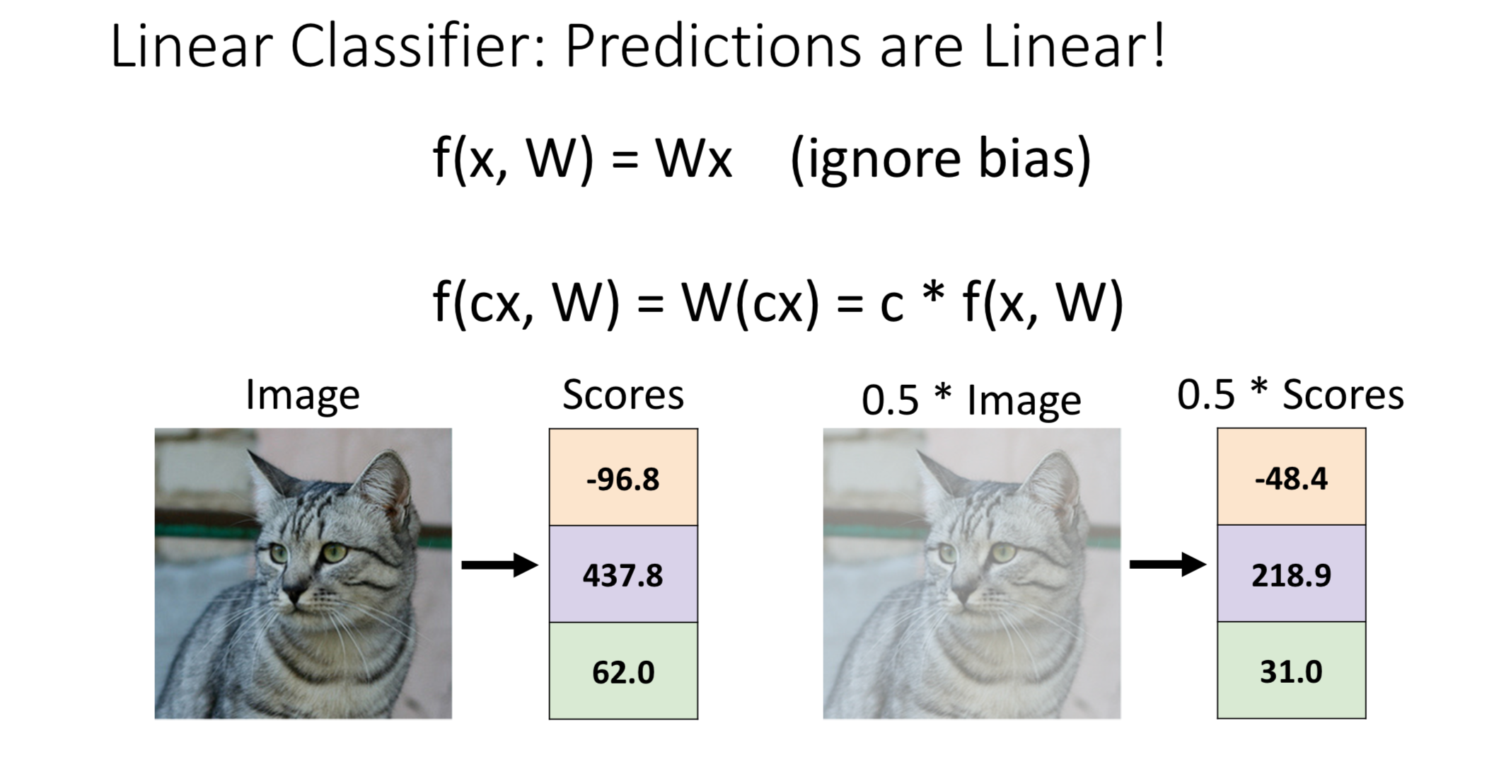
2. Prediction are Linear

If the linear classifier is

$$f(x_i,W)=Wx$$

then

$$f(c{x}_i,w)=W(cx)=c\cdot f(x_i,W)$$

Making each RGB value half in the original image will make the fades but preserve the original color

From the human perspective, the two images are almost the same, but linear classifier gives only half of the score, this may affects the function of loss function

Visual Viewpoint

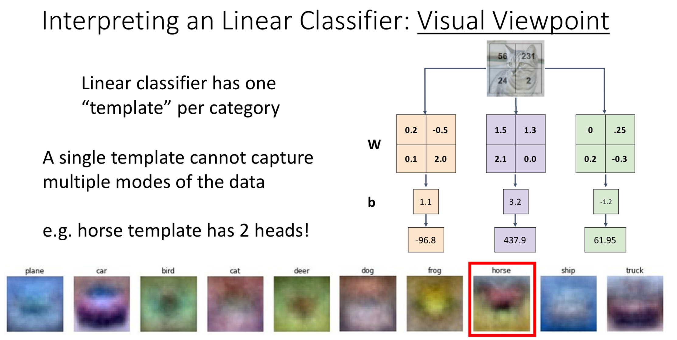
In visual viewpoint, we don’t stretch the input into vector ($3072\times 1$). Instead, we maintain its shape ($32\times 32\times 3$). Now, we calculate score to each label separately, we’ll then have weights in the shape $32\times 32\times 3$

We call the weights in this shape a template, it represent how linear classifier thinks the “average image” of this label looks like

Looking at the slide above, you can see the horse picture has two head, since in the dataset there are horse facing left and horse facing right

Thus one template per label can’t represent all kinds of images in this label, we’ll solve this problem using neural network in the neural network lectures

Geometric Viewpoint

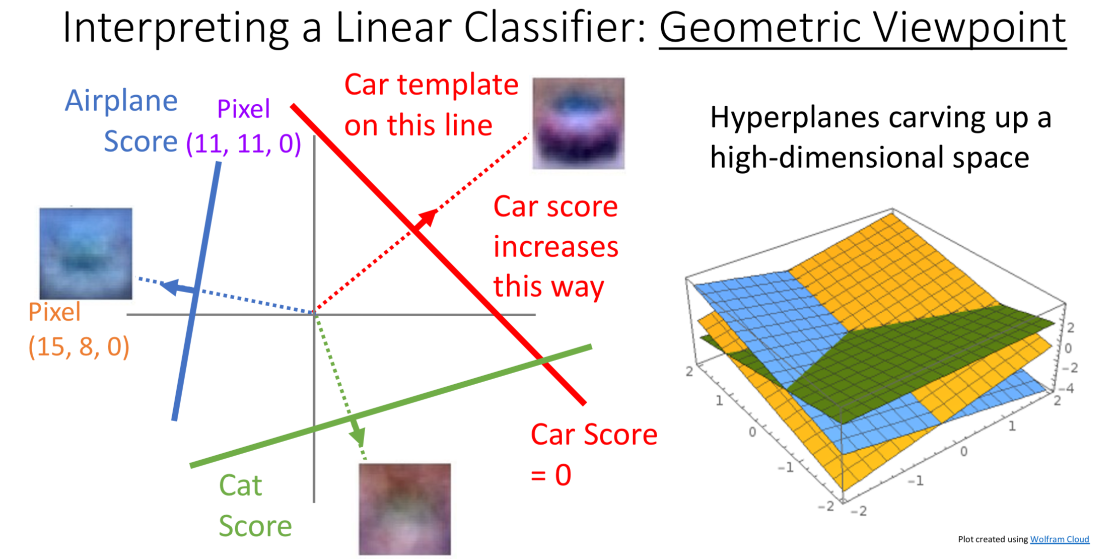
1. Thinking of Input Images as Points in Space

In the geometric viewpoint, we treat each feature of the image (such as a pixel’s RGB value) as a dimension in space. Every image corresponds to a single point in this multi-dimensional space. Images that share similar characteristics will appear as points that are positioned close to each other in this mathematical space.

2. Linear Classifier as a Plane in Space

The linear classifier can be thought of as a plane defined by the equation $ax+by+cz=\text{score}$ in this space. When the plane moves in the direction of its normal vector, the score increases, and vice versa. This geometric relationship allows us to understand how the classifier assigns different scores to different points in the feature space.

3. Making Decisions

By using mathematical methods, we can calculate the “distance” from the point that represents the image to the linear classifier plane (defined by $ax+by+cz=\text{final score}$). This distance tells us how close the image is to each possible class label.

With the distance values between the image and every class label, we can determine which class the image should be classified into by selecting the class with the smallest distance or highest score.

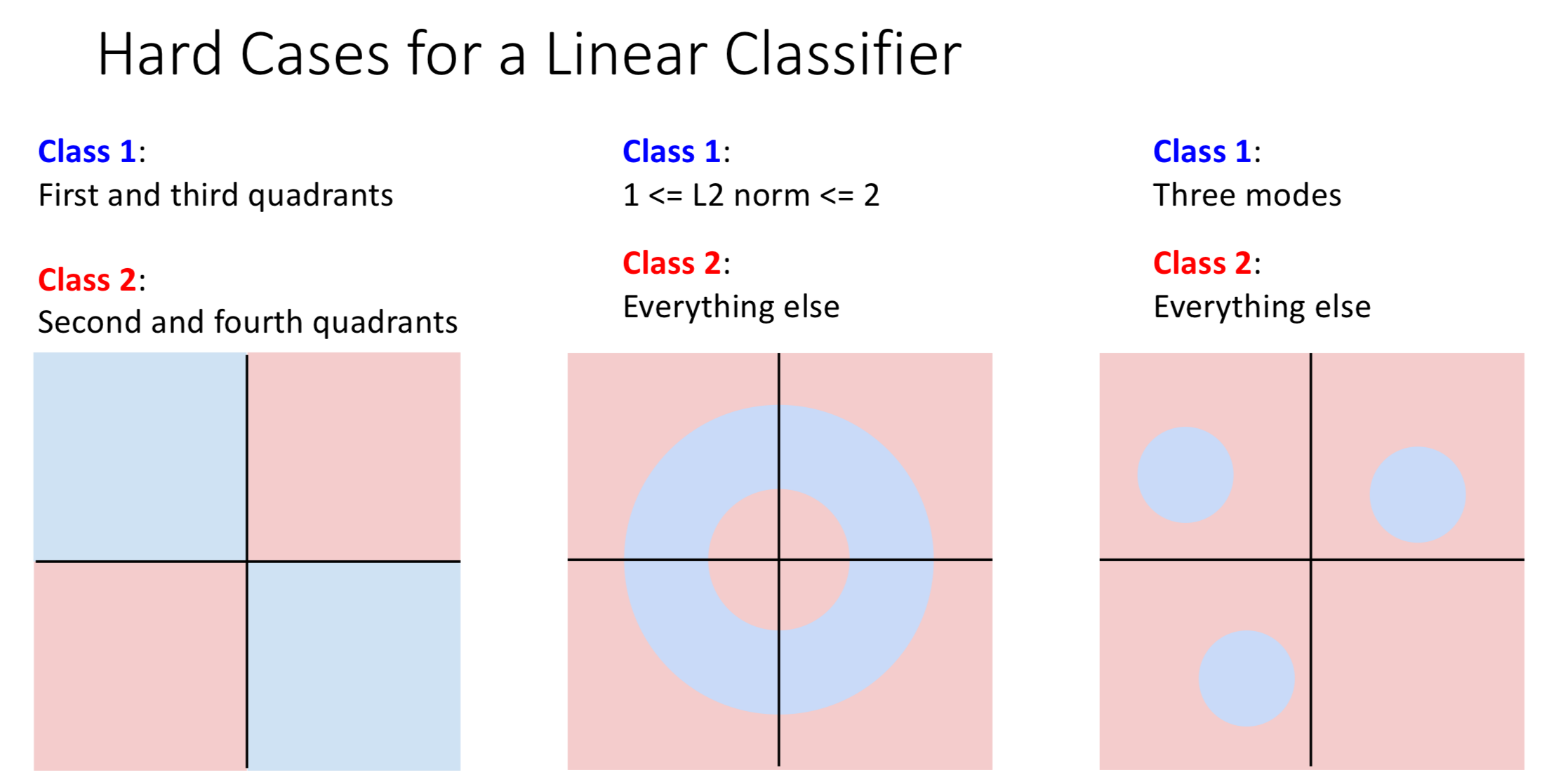
Hard Cases for Linear Classifier

The three cases in the picture below show the limitation to linear classifier. These cases use two dimension to explain the idea, but in reality the number of dimension will be much larger

Explanation: For these three cases, we can not use a straight line (linear classifier) to divide the region separating different classes