D-DL4CV-Lec13b-AttentionLayer

Simplified Attention Layer

1. Input

• Query Vectors: $q\in {\mathbb{R}}^{D_Q}$
• Input Vectors: $X\in {\mathbb{R}}^{N_X\times D_X}$
• Assumption: For the dot product to be valid, we must have $D_Q=D_X$

2. Computation

1. Alignment Scores ($e$): Measures the similarity between $q$ and each row $X_i$

$$e=\frac{q{X}^{\top }}{\sqrt{D_Q}}(\text{Shape: }1\times N_X)$$

2. Attention Weights ($a$): Normalize scores into a probability distribution.

$$a=\text{softmax}(e)(\text{Shape: }1\times N_X)$$

3. Output Vector ($y$): A weighted sum of the inputs.

$$y=aX=\sum _{i=1}^{N_X}{a}_i{X}_i(\text{Shape: }1\times D_X)$$

Why Scale by $1/\sqrt{D_Q}$?

As $D_Q$ grows, the variance of the dot product increases. Large scores push the softmax into regions with extremely small gradients (“saturation”), leading to vanishing gradients during backprop. Scaling keeps the variance near 1.

---

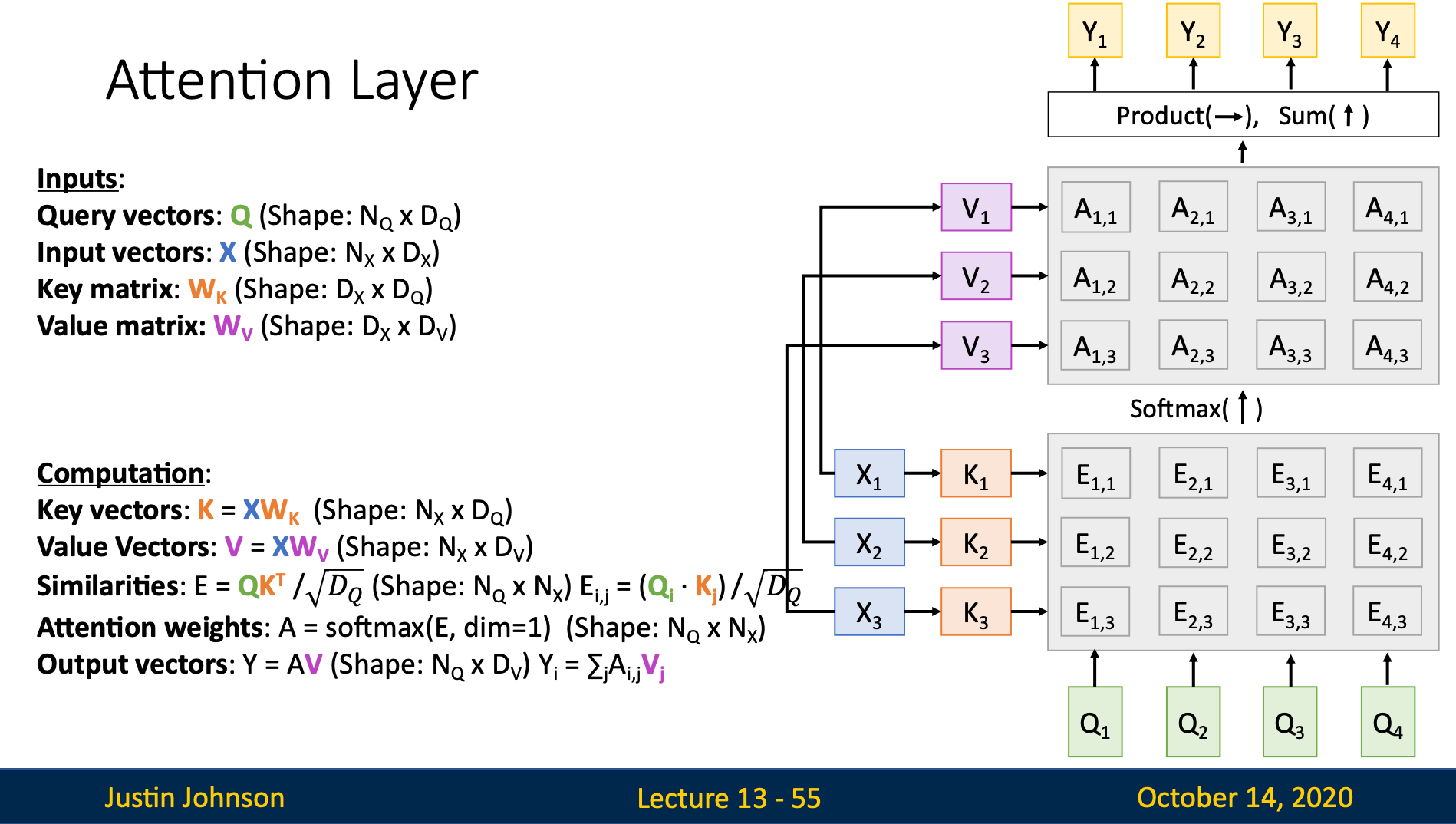
Standard Attention Layer

1. Introduction

In practice, we don’t just use the raw input $X$. We project it into different spaces for “matching” (Key) and “extracting” (Value).

2. Input

• Query Matrix: $Q\in {\mathbb{R}}^{N_Q\times D_Q}$
• Input Matrix: $X\in {\mathbb{R}}^{N_X\times D_X}$
• Weight Matrices:
  • $W_Q\in {\mathbb{R}}^{D_Q\times d_k}$ (Projects query to internal dim)
  • $W_K\in {\mathbb{R}}^{D_X\times d_k}$ (Projects input to key space)
  • $W_V\in {\mathbb{R}}^{D_X\times d_v}$ (Projects input to value space)

3. Computation Pipeline

1. Linear Projections:

$$Q^{\prime }=Q{W}_Q,K=X{W}_K,V=X{W}_V$$

2. Similarity Matrix ($E$):

$$E=\frac{Q^{\prime }{K}^{\top }}{\sqrt{d_k}}(\text{Shape: }{N}_Q\times N_X)$$

Each $E_{i,j}$ is the score between the $i$-th query and $j$-th key.

3. Attention Weights ($A$):

$$A=\text{softmax}(E,\text{dim}=1)(\text{Shape: }{N}_Q\times N_X)$$

4. Final Output ($Y$):

$$Y=AV(\text{Shape: }{N}_Q\times d_v)$$

This is a “row-wise” combination: each row $Y_i$ is a weighted sum of all rows in $V$, i.e.,

$$Y_i=\sum _j{A}_{i,j}{V}_j$$

4. Query, Key, and Value Vectors

We can observe that both alignment scores and output vector use input vectors in its computation. However, they serve for different purposes

1. in alignment scores: it serves purpose for pattern matching
2. in output vector: it acts as actual info contain in input

Since they serve for different purposes, we can use learnable parameters to optimize them for separate use

Key Vector

$$K=X{W}_K$$

The key matrix $W_K$ learns what features do the query vector wants to match, then $W_K$ will extract desired features from the original input vector $X$

Value Vector

$$V=X{W}_V$$

The input vector mix all the features in the image together, value matrix learns to extract valuable features from the image to send to the next layer

Query Vector

It contains the current context we have. We can think of it as saying: “Based on the context in the first $t-1$ periods, what part of the input $X$ should I look at to generate the next output”

5. Deep Dive: Training vs. Inference

Training

We use Teacher Forcing. Since the entire target sequence is known, we can compute all Queries ($Q$) at once. The “dependence on previous step” is bypassed by using the ground truth.

Inference (Generation)

We must process Autoregressively. The Query for step $t$ depends on the output generated at $t-1$. Here, parallelization only happens across the “Input” side ($K$ and $V$ are static), not the “Query” side.