D-DL4CV-Lec11a-LearningRateSchedule

Constant Learning Rate

Introduction

This is the learning rate schedule which we’ve stick in the previous lectures, which can be interpreted as:

$${\alpha }_t={\alpha }_0$$

That is, the learning rate doesn’t changes as the training progress, but how can we efficiently choose this specific ${\alpha }_0$

Efficient Learning Rate Search Strategy

Core Strategy

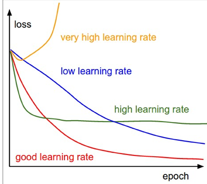
Search from large → small learning rates

Why It Works

• Large LR = Fast training → Test multiple candidates quickly
• Decreasing LR → Loss curves become progressively smoother
• Stop when good enough (close to “good learning rate” in the image) or time runs out

Process

1. Coarse Search: Start large (0.1) → decrease (0.01, 0.001, 0.0001)
2. Fine Search: Grid/random search around best range found

Benefits

• Time-efficient elimination of poor candidates
• Focus resources on promising ranges only

---

Learning Rate Decay

Step Decay

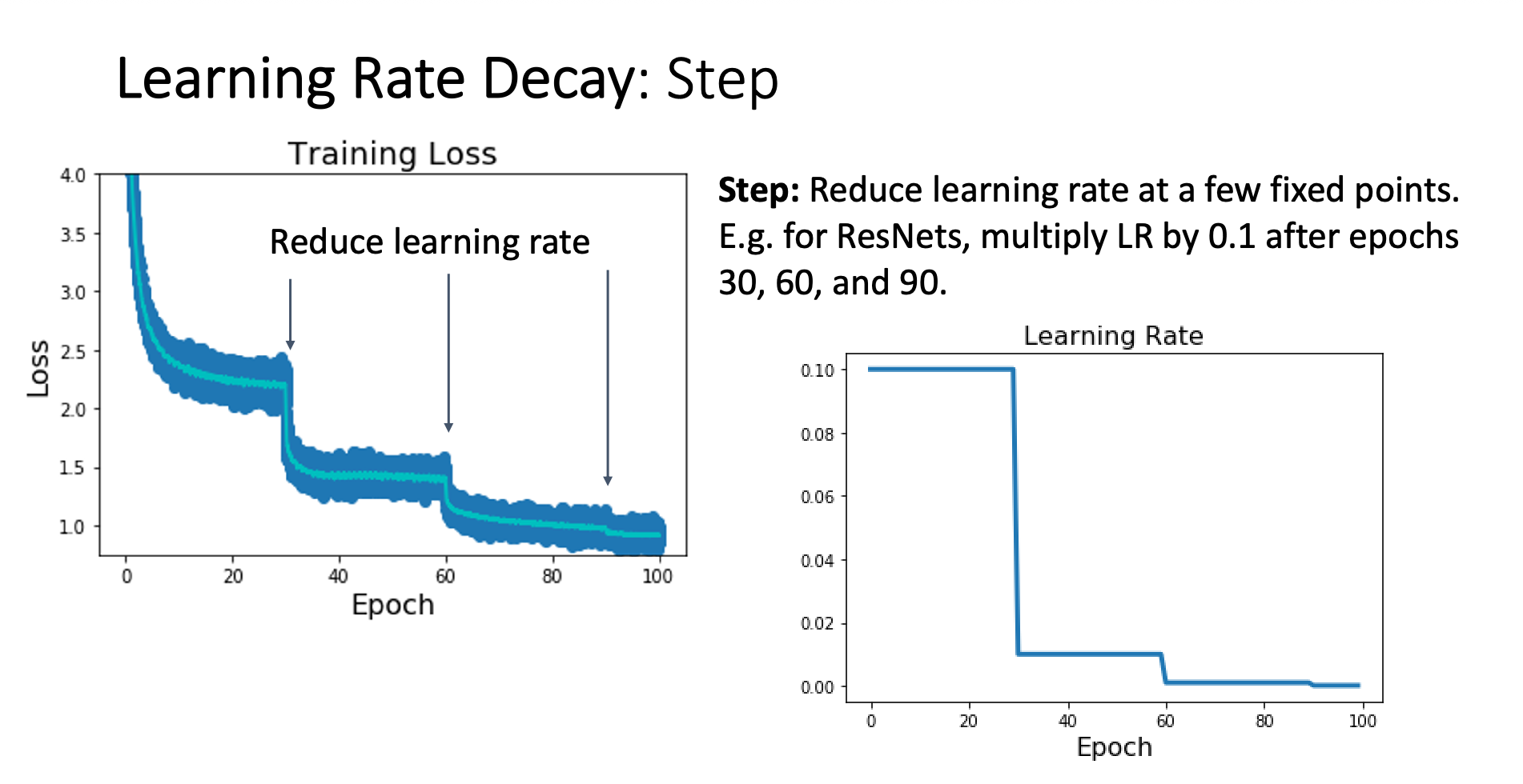
Strategy

Reduce learning rate at a few fixed iterations decided by the researcher, mostly we multiply the previous LR by 0.1

Pros and Cons

Pros:

1. Easy to implement and understand
2. Allow aggressive learning initially, then subtle update in later stages

Cons:

1. Too many hyperparameters to tune (${\alpha }_0$, when to reduce LR, reduction factor)

Cosine Decay

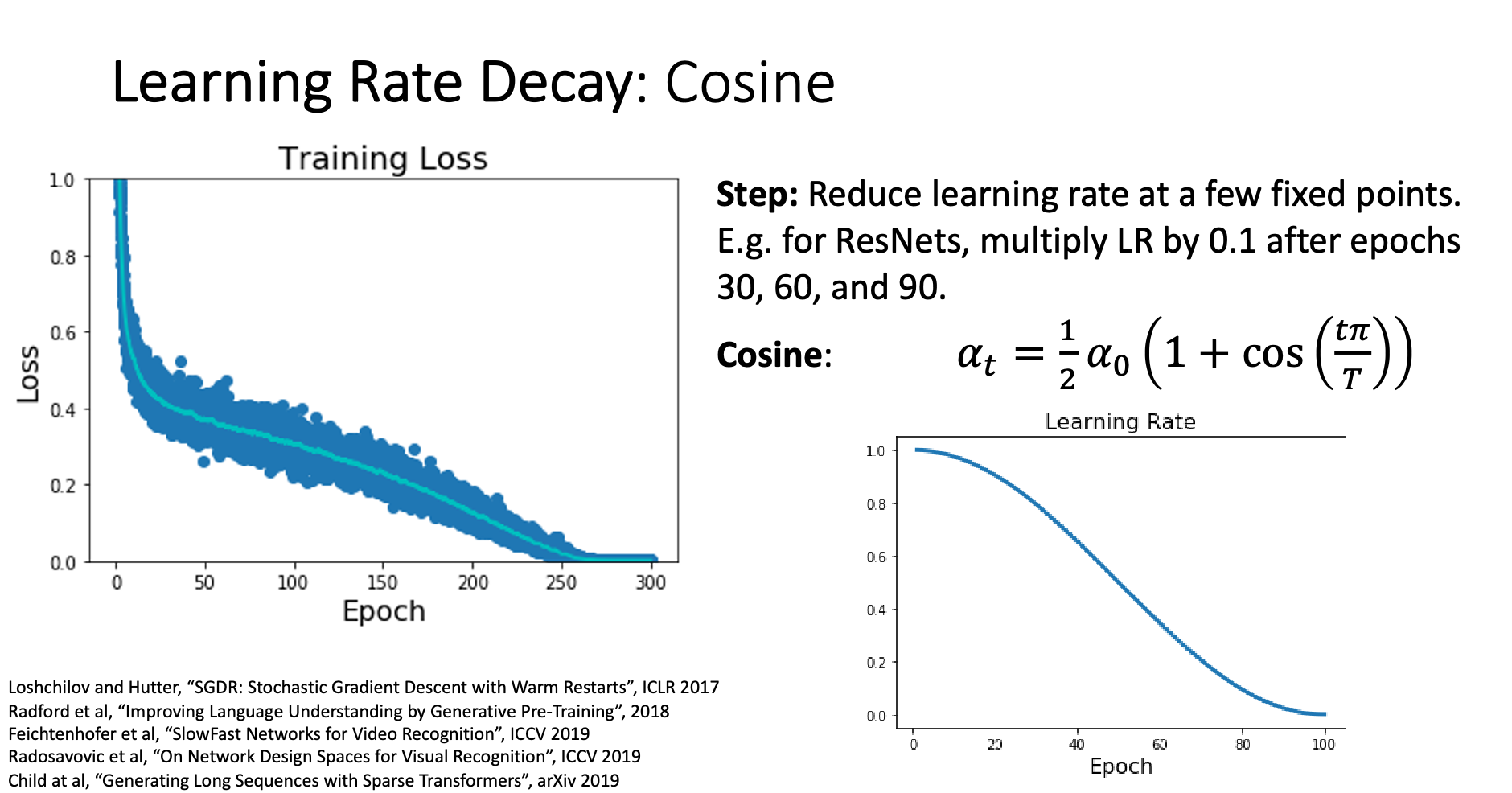
The learning rate decay using the following formula

$${\alpha }_t=\frac{1}{2}{\alpha }_0\left(1+\cos \left(\frac{t\pi }{T}\right)\right)$$

Linear Decay

The learning rate decays linearly

$${\alpha }_t={\alpha }_0\left(1-\frac{t}{T}\right)$$

Inverse Sqrt Decay

This decay method is used by “Attention is all you need”

$${\alpha }_t=\frac{{\alpha }_0}{\sqrt{t}}$$

---

How Long to Train?

When to Stop Training?

Stop when the validation accuracy starts to decrease

This indicates overfitting - the model is memorizing training data rather than learning generalizable patterns.

How to Get the Best Model?

The final model might not be the best one due to overfitting.

Process:

1. Save model snapshots regularly during training
2. After training, select the snapshot with highest validation accuracy

Example:

Epoch 30: Val Acc = 90% ← Use this model
Epoch 40: Val Acc = 89% 
Epoch 50: Val Acc = 87% ← Stop here

---

Tricks

1. SGD+Momentum → Use LR decay
2. More complicated optimization algorithm → Use constant LR is enough