D-DL4CV-Lec06-Backpropagation

Why We need Backpropagation?

Why we need backpropagation?

We’ve learned in lecture 4 that we need the gradient of the loss to optimize our model. If we directly compute the gradient by definition, it will be a disaster

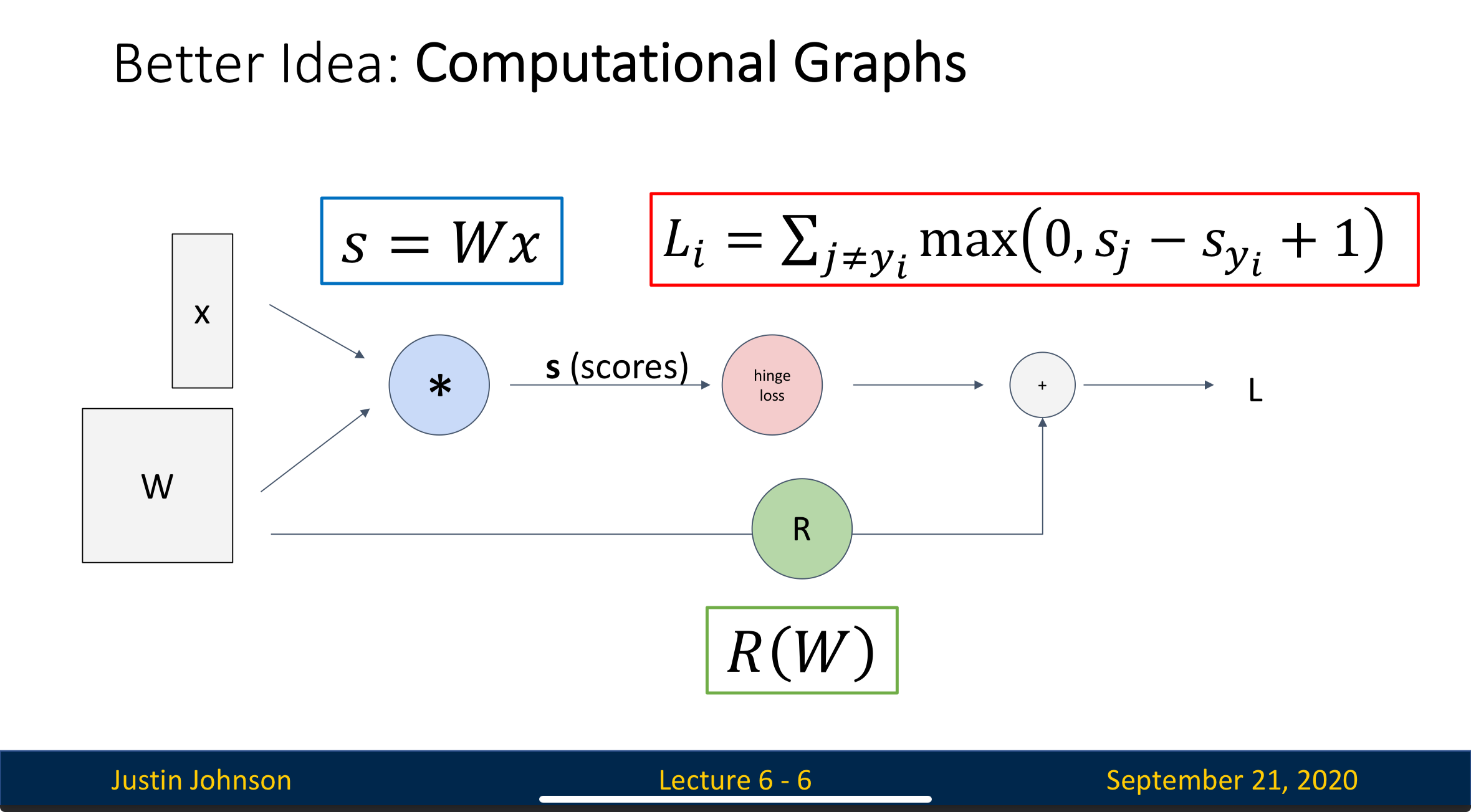
Take SVM as example:

$$\begin{array}{rl}s& =f(x,W)=Wx\\ L_i& =\sum _{j\ne y_i}\max (0,s_j-s_{y_i}+1)\\ & =\sum _{j\ne y_i}\max (0,W_{j,:}x-W_{y_i,:}x+1)\\ L& =\frac{1}{N}\sum _{i=1}^N{L}_i+\lambda \sum _k{W}_k^2\\ & =\frac{1}{N}\sum _{i=1}^N\sum _{j\ne y_i}\max (0,W_{j,:}x-W_{y_i,:}x+1)+\lambda \sum _k{W}_k^2\\ & ⟹{\nabla }_{W}L={\nabla }_W\left(\frac{1}{N}\sum _{i=1}^N\sum _{j\ne y_i}\max (0,W_{j,:}x-W_{y_i,:}x+1)+\lambda \sum _k{W}_k^2\right)\end{array}$$

This simple linear classifier with SVM loss function already has this complex gradient formula, how about more complex models? Hence, a better way to calculate gradient is necessary

Backpropagation is exactly an efficient way to help us calculate the gradient

---

Simple Introduction to Backpropagation

Computational Graph

To understand backpropagation, the first thing we need to do is to turn the process of neural network into a computational graph

The input data goes from the left of the graph to the right to produce output, this process is called “forward pass”

Process

Step 1: Forward Pass

The data flows forward through the network, producing a prediction

Step 2: Loss Calculation

The prediction is then put into the loss function to produce the loss

Step 3: Backward Pass

The algorithm then works backward from the output to the input. During the process, we can efficiently calculate the gradient of loss with respect to the weight of the layer

The gradient tells us how much each weight contributes to the total loss, i.e. $\partial L/\partial w$

Step 4: Weight Update

We can then update the weight based on the gradient

How Data is Processed in Backward Pass

Concepts

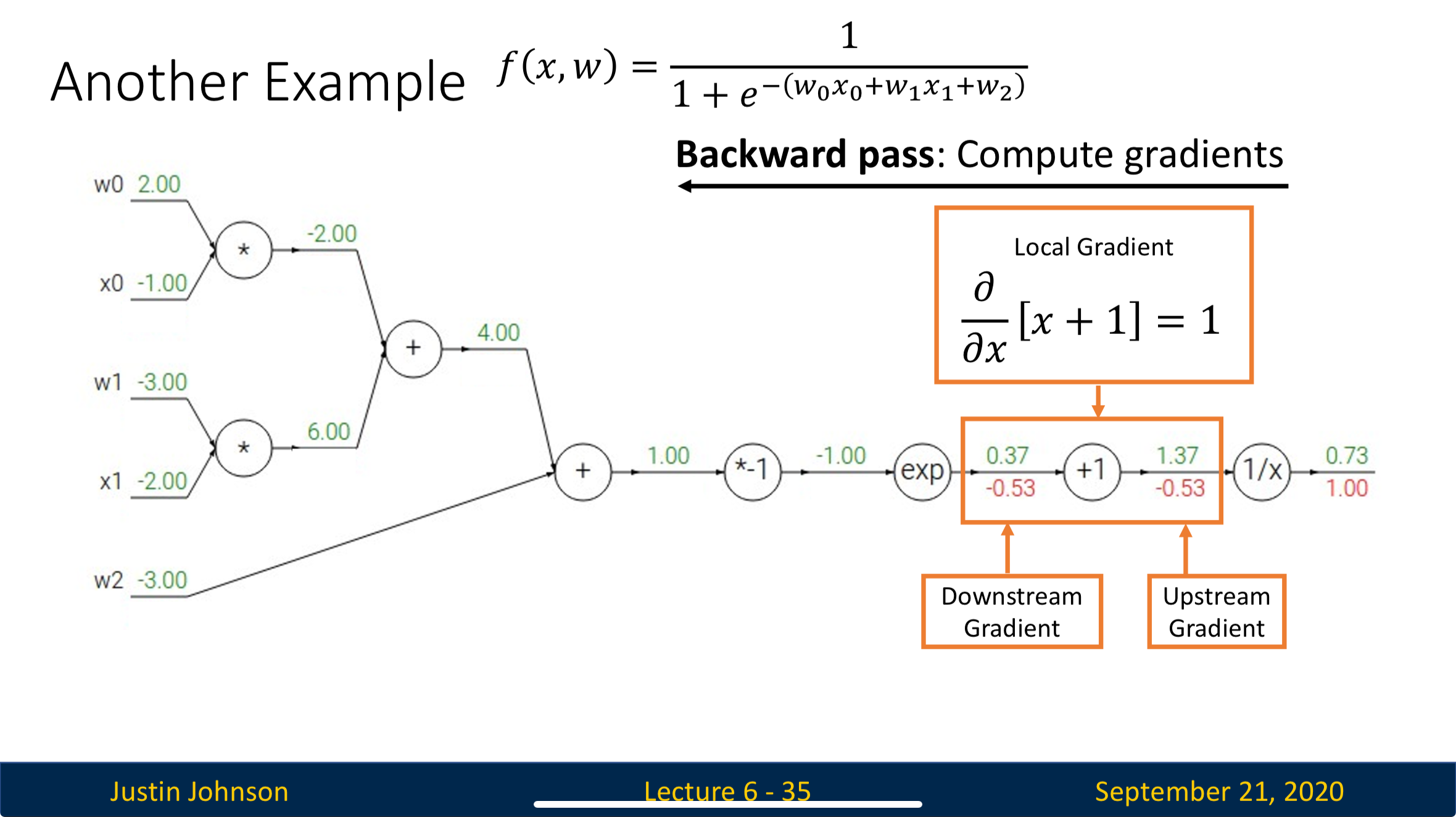
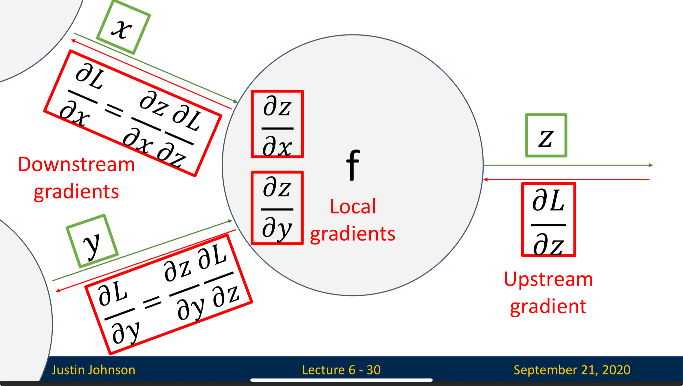
Upstream Gradient: The gradient flows into the neuron, representing how loss changes as the neuron’s output ($z$) change

Local Gradient: The gradient that represent how much the neuron’s output changes when its input changes

Downstream Gradient: The gradient that flows out of the neuron, which is the upstream gradient of the next neuron

Process

We’ll focus on this single neuron

1. The neuron receives the upstream gradient, we don’t need to know how it is calculated since it’s the task of previous neuron
2. Using the input and output of the neuron when conducting forward pass, we can get the local gradients
3. By multiplying upstream gradient with local gradient, we can get the downstream gradient, which we’ll pass to the next neuron

By process above, we conclude that

$$\text{downsteam gradient}=\text{local gradient}\cdot \text{upstream gradient}$$

Define Complex Primitives Instead of Simple Ones

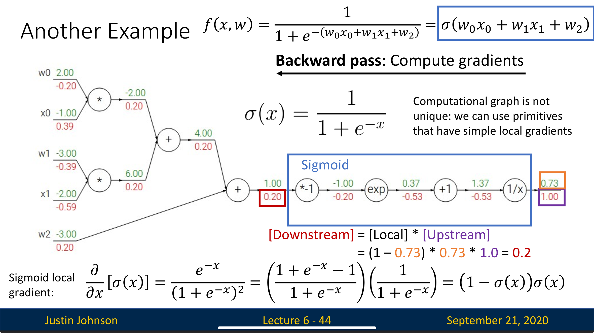
We usually combine several successive simple primitives into one complex primitive to decrease computation since the more neuron you have, the more dot product computation you’ll need

Take the computational graph below as example: If we combine the four circled neurons into one sigmoid neuron, then we’ll only need to compute once to complete the computation that we previously need four computation to achieve

---

Backpropagation in Vector-Valued Function

Dimensions

1. Upstream Gradient $\in {\mathbb{R}}^Z$
2. Downstream Gradient $\in {\mathbb{R}}^X$
3. Local Gradient $\in {\mathbb{R}}^{Z\times X}$

Jacobian

For $y\in {\mathbb{R}}^n$ and $x\in {\mathbb{R}}^m$, then $\frac{\partial y}{\partial x}$ is $m\times n$ matrix with ${\left(\frac{\partial y}{\partial x}\right)}_{i,j}=\frac{\partial y_j}{\partial x_i}$

Trap When Calculating Gradient

Concept

There are two ways (implicit, explicit) to calculate gradient, we prefer implicit multiplication over explicit due to memory efficiency

$$\text{downsteam gradient}=\text{local gradient}\cdot \text{upstream gradient}$$

Explicit Jacobian Formation: In this method, we first form the Jacobian matrix (${\mathbb{R}}^{Z\times X}$), then do matrix vector multiplication to get the downstream gradient

Implicit Multiplication: In this method, we never actually form the entire Jacobian matrix. Instead, we directly compute $\text{local gradient}\cdot \text{upstream gradient}$ element-wise without storing intermediate matrices

Explanation

When the number of features gets large, $Z\times X$ will be a huge number. If we choose to do the computation explicitly, we’ll need to store $Z\times X$ values, which exceed the GPU memory.

On the other hand, calculate it implicitly won’t create any intermediate matrix, making this method memory efficient

Also, most of the time, the Jacobian matrix is sparse, meaning most of the entries are useless, which waste a lot of memory

How to understand Backpropagation of High-Dimensional Input & Output

Hard to explain, see UMich Lecture 6: Backpropagation start from 47:50

---

Backpropagation: Another View

Reverse-Mode Automatic Differentiation

    f_1      f_2      f_3      f_4
x_0 ---> x_1 ---> x_2 ---> x_3 ---> L

For the diagram above, we can calculate the partial derivatives of loss with respect to $x_i$ by the formula below:

$$\frac{\partial L}{\partial x_0}=\left(\frac{\partial x_1}{\partial x_0}\right)\left(\frac{\partial x_2}{\partial x_1}\right)\left(\frac{\partial x_3}{\partial x_2}\right)\left(\frac{\partial L}{\partial x_3}\right)$$

Since matrix multiplication is associative, we can calculate it in any order. If we multiply from right to left, we can avoid doing matrix-matrix multiplication, which is time inefficient. Instead, calculating from right to left gives us matrix-vector multiplication

Forward-Mode Automatic Differentiation

  f_1      f_2      f_3      f_4
a ---> x_0 ---> x_1 ---> x_2 ---> x_3

For the diagram above, we can calculate partial derivatives of $x_i$ with respect to $a$ by the formula below:

$$\frac{\partial x_3}{\partial a}=\left(\frac{\partial x_0}{\partial a}\right)\left(\frac{\partial x_1}{\partial x_0}\right)\left(\frac{\partial x_2}{\partial x_1}\right)\left(\frac{\partial x_3}{\partial x_2}\right)$$

This is seldom seem in machine learning. Instead, it is often seen in other computer science fields

Hessian-Vector Products via Backpropagation

The Problem

Computing the full Hessian matrix (second derivatives) is expensive - it requires $O(n^2)$ memory and computation for n parameters. But often we only need the Hessian multiplied by a vector v, not the full matrix.

The Solution: A Clever Trick

Instead of computing the Hessian directly, we can use backpropagation twice:

1. First backprop: Compute the gradient $dL/d{x}_0$
2. Second backprop: Treat $(dL/d{x}_0)v$ as a new “loss” and backpropagate through it

The Key Insight

The mathematical trick is:

$$\frac{{\partial }^{2}L}{\partial x_0^2}v=\frac{\partial }{\partial x_0}\left[\frac{\partial L}{\partial x_0}\cdot v\right]$$

This means: “The Hessian-vector product equals the gradient of the dot product (∂L/∂x₀)·v”

The Process

    f_1      f_2    f_2^T         f_1^T          *v
x_0 ---> x_1 ---> L ----> dL/dx_1 ----> dL/dx_0 ---> (dL/dx_0)v

When we backpropagate through this extended computation graph, we get the Hessian-vector product $({\partial }^{2}L/\partial x_0^2)v$ as the gradient with respect to $x_0$.

Why This Works

Backpropagation automatically applies the chain rule. By making $(dL/d{x}_0)v$ our “input” backprop computes its derivative with respect to $x_0$, which is exactly the Hessian-vector product we wanted!